Therefore, we use the following statement to generate the column list for us. The following command will open your own schema on the demo system. Therefore, we can think that 0 represents orange, and 1 refers to apple. This notebook is an extension from the Python Programming and Numerical Methods - A Guide for Engineers and Scientists, the content is also available at Berkeley Python Numerical Methods. If we only plot the first two features, i.e. A dataset is a dictionary-like object that holds all the data and some metadata about the data. Using these existing datasets, we can easily test the algorithms that we are interested in. For SVM, two most important parameters are C and gamma. In the case of supervised problem, one or more target variables are stored in the .target member. Copy the statement below in your SQL Client. If we can, we always want to plot the data out first to explore it. This tutorial is designed to work with the Free Trial System.Ensure you have access to the public demo system. This table will be used to evaluate our results. Else sign up here to get access to the demo system hosted by Exasol for testing the data and scripts in this tutorial. If you find this content useful, please consider supporting the work on Elsevier or Amazon! So the first parameter we hand over to the UDF is the path to our model in BucketFS. The use of the different algorithms are usually the following steps: Step 1: initialize the model NOTE: Please note that schema is only set for the current session. 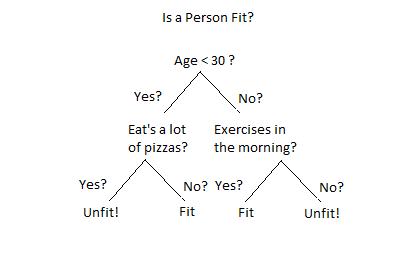 Introduction to Machine Learning, Appendix A. The API is quite simple, for most of the algorithms they are similar. Based on the above discussion, we should choose the red solid line which matches our intuition.
  There are many different packages in Python that can let you use different machine learning algorithms really easy. In the following step we will also define the details for accessing the content in this bucket. We start by loading some pre-existing datasets in the scikit-learn, which comes with a few standard datasets. With the following statement, we test the connectivity to the database: Now that the connection is opened, we can move on to the next step - Examine the data. Linear Algebra and Systems of Linear Equations, Solve Systems of Linear Equations in Python, Eigenvalues and Eigenvectors Problem Statement, Least Squares Regression Problem Statement, Least Squares Regression Derivation (Linear Algebra), Least Squares Regression Derivation (Multivariable Calculus), Least Square Regression for Nonlinear Functions, Numerical Differentiation Problem Statement, Finite Difference Approximating Derivatives, Approximating of Higher Order Derivatives, Chapter 22. We can first calculate features for each apple and orange and save it into the feature matrix as shown in the above figure. This is the design of the SVM algorithm, it first forms a buffer from the boundary line to the points in both classes that close to the line (these are the support vectors, where the name comes from). It contains multiple tables filled with training and test data. Now lets use scikit-learn to train a SVM model to classify the different species of Iris.
 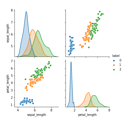 As shown in the following figure, if we have a new data point (the blue dot), then the black dotted line model will make the wrong decision. Since we only have two classes, this problem is usually called binary classification problem. Additionally, we create a confusion matrix that displays how the instances were classified. As mentioned in the step before, we need all the columns as input parameters for our script and do not want to type them manually. If we plot out the support vectors, it shows in the following figure. Four features were measured from each sample: the length and the width of the sepals and petals, in centimetres. As we have 170 measures to take into account, manually typing the list of input and output parameters would be quite some work. Most people will choose the red solid line, because it is in the middle of the gap between the two groups. The output of this statement is a list of all the columns which can copy into our script at the right places before creating it. If there's anything we can improve on, let us know. For the testing dataset, which is not used in training at all, it is only saved for evaluation purposes. Once you have installed pyexasol, we can start writing our script by specifying the connection details for the Exasol demo system that we will use later on. The classification problem essentially is a problem to find a decision boundary, either a straight line or other curves, to separate them. Afterward, execute the statement to create the table TEST_PREDICTIONS. Enter the credentials you received by email. BucketFS Bucket: showcase. The most popular package for general machine learning is scikit-learn, which contains many different algorithms. Now we see how we can train a model to do the classification in Python, there are also many other models that you can use in scikit-learn, we leave this for you to explore. def test(X, class_col_name, model_path=None): X_data = X.loc[:, X.columns != class_col_name], df = ctx.get_dataframe(num_rows='all', start_col=num_non_data_cols), y_pred = test(df, class_col_name='CLASS', model_path=classifier_path), df_pred = (pd.DataFrame(y_pred, columns=['CLASS_PRED'])).join(df), '/buckets/bucketfs1/demo_ida/classifier3.pkl', CREATE OR REPLACE TABLE IDA_TEST_PREDICTIONS AS, SELECT IDA_TEST_MODEL('{EXASOL_BUCKETFS_PATH}/{model_file}', {", # Define cost function from the problem description. This tutorial serves the purpose of trying out user-defined functions (UDFs) on an available machine learning model with a test dataset. Therefore, the model which has a line close to the middle of the gap and far away from both classes are better ones. The following function plot the decision boundary. Classification is a very common problems in the real world. As shown in the following figure, the black dotted line has a narrow buffer while the red solid line has a wider buffer. If you are interested in a full end-to-end demonstration of how the machine learning techniques can be directly applied in Exasol, refer to our Data Science GitHub repository. Copy the script below in your SQL Client. We are now prepared to run the data science model for prediction and evaluation on the data. Also, the boundary between these classes are fairly linear, thus all we need to do is to find a linear boundary between them. The demonstration does not require a deep understanding of data science or machine learning methods.
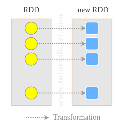
 We can see the linear boundaries found by the SVM for the 3 classes are generally good, and can separate most of the samples. Therefore, we use the system tables containing the column names and column types to generate these for us. Exasol ships with a default language container for Python 3.6 that can be used to run Python UDFs out of the box in the database.
 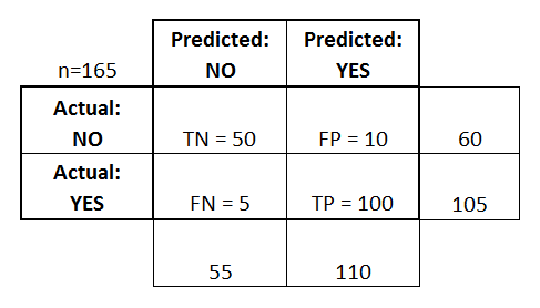 < 25.1 Concept of Machine Learning | Contents | 25.3 Regression >. Object Oriented Programming (OOP), Inheritance, Encapsulation and Polymorphism, Chapter 10. Afterward, execute it to create the script.If you are using DbVisualizer, you have to disable Parameterized SQL before executing a script containing '&' - Symbols. To connect to the system, you can use the SQL Client of your choice. Lets again see an intuitive example, the classification of a group of apples and oranges. Refer to the Exasol Script Language GitHub Repository for instructions. Then the problem becomes given a set of these support vectors, which line has the maximum buffer. If you're running inside a Jupyter notebook, add an exclamation mark before the statement. The UDF TEST_MODEL takes the path to our model and all the input columns as input parameters. Next, execute the above statement and copy the output to the script below at the two places where it says
 . Ordinary Differential Equation - Initial Value Problems, Predictor-Corrector and Runge Kutta Methods, Chapter 23. The schema we are working with is called "IDA". We can plot it as a scatter plot with different symbols for different classes. After running the above evaluation script, the following results should be displayed. Step 3: predict on the new data using the predict function. The following table provides you with the details on connecting to an SQLclient and Python environment. If you haven't already, sign up for an account on this page in the Get a test account for ExaCloud section. Therefore if you reconnect to the system, you have to execute this statement again. This language container includes some commonly used data science modules. The data is publicly available in the IDA 2016 Challenge dataset from the Industrial Challenge at the 15th International Symposium on Intelligent Data Analysis (IDA) in 2016. BucketFS Service: bucketfs1
In the process, we demonstrate that there is no need to export data from Exasol to a different system for training and testing machine learning models. We wont go into the details here, but a good advice is that before you use the model, always try to understand what these parameters are to get a good model. Exasol recommends DbVisualizer in the Pro version, an open source alternative is the tool DBeaver. The text is released under the CC-BY-NC-ND license, and code is released under the MIT license. As a first step, we will create a connection to the system and get familiar with the table structures. In this step we will create a Python UDFcalled IDA_TEST_MODEL, which will be used to predict results for the test data (i.e., whether a failure is an APS failure or not) in the next step. In this case, we use a small helper statement to do the work for us. Lets look at the following figure, and ask the question which line boundary is better? The black dotted line or the red solid line? Errors, Good Programming Practices, and Debugging, Chapter 14. Please select a platform to see relevant administration content. color and texture, we may see something as below: We can see that the blue dots (apples) and orange square (oranges) falls on the different parts in the figure. In the below sections, both these approaches are presented side by side to give you a better understanding and to help you choose the preferred approach. This data is stored in the .data member, which is a n_samples, n_features array. By joining the predicted class labels to the test data, we ensure that the predicted and real class labels remain properly ordered / linked for evaluation as we don't have a smaller set of columns that uniquely identifies each row. That way, you can create a custom UDF environment tailored to your needs. We use a cost function which we call ida_cost() as a performance metric, which implements the cost function specified in the problem description. This intuition from us need to be formalized into a way that the computer can do this. We define a few variables that contain information about the information about where to find the model that we want to test in the BucketFS. Each of them represent a class. In the below commands, replace with your username and run the commands. Depending on your package manager, you can either use. For this demo, we will use a dataset on the publicly available Exasol demo system. Everything can be done using UDFs directly inside Exasol where the data is stored. Lets prepare the feature matrix \(X\) and also the target \(y\) for our problem. Both approaches will give us the same results in the end, the advantage of the latter one is that it allows you to play around with dataframes inside Python and lets you visualize results more easily. With the confusion matrix and the total cost, we can now compare our model to others. To connect to Exasol, install the pyexasol package in your local Python environment. As we will use an already trained model, we will only need the test data in a normalized format. Replace the schema name with your username in order to create the UDFs in your own schema. The iris dataset consists of 50 samples from each of three species of Iris (Iris setosa, Iris virginica and Iris versicolor). In the resulting table IDA_TEST_PREDICTIONS, we now have a column with the prediction made by our model CLASS_PRED and the actual label as the ground of truth in the column CLASS. We can plot the decision boundary for the model. We will focus on the last steps, which is, running the model on the test data and evaluating its performance (steps 3 and 4 in the image below). If you need further libraries not included in the default container or you want to use another version of Python, Exasol allows you to create your own script language containers including these. The above print out from the fit function is the parameters used in the model, we can see that usually for a model there are many different parameters that you may need to tune. To disable Parameterized SQL, navigate to SQL Commander --> SQL Commander Options and uncheck Parameterized SQL option. You can easily install scikit-learn use a package manager. Then, execute the statement above and copy the output in the script below where it says . Now lets use the predict function on the training data, usually we dont do this, we need to split the data into training and testing dataset. We will compare these two columns in the next step to evaluate how well our model performed. One popular way to do the job is the support vector machine (SVM). Now that we've got an impression of the data, we will move on to the next step of preparing our environment for the creation of UDFs. The data is always a 2D array, shape (n_samples, n_features), although the original data may have had a different shape. For this demo, we use a Jupyter notebook running with Python 3.6. For example, you can use an artificial neural network (ANN) to do the same job (hint: use the MLPClassifier for the ANN classifier). Step 2: train the model using the fit function Since we have 5 features in the figure, it is not easy to visualize it. "select count(*) from IDA.IDA_TEST_TRANSFORMED", "select * from IDA.IDA_TEST_TRANSFORMED LIMIT 5", # Close Exasol connection, we will open a new one in the next step, -- Open your own schema, we will create our scripts in this schema later on, "/buckets/{EXASOL_BUCKETFS_SERVICE}/{EXASOL_BUCKETFS_BUCKET}", # Filesystem-Path to the read-only mounted BucketFS inside the running UDF Container, # Add class predictions as first column of test DataFrame, # Read one line of the dataset to get the structure, "SELECT * FROM IDA.IDA_TEST_TRANSFORMED LIMIT 1", ###column_types = ["VARCHAR(3)"] + ["DECIMAL(18,2)"] * (len(column_names)), ###column_desc = [" ".join(t) for t in zip(column_names, column_types)], # Create script output column descriptions, CREATE OR REPLACE PYTHON3 SET SCRIPT IDA_TEST_MODEL(CLASSIFIER_PATH VARCHAR(200), {", ".join(column_desc)}. Getting Started with Python on Windows, Python Programming and Numerical Methods - A Guide for Engineers and Scientists. Here for simplicity, we just have a look of the results on the training data we used. The tuning of the algorithm is basically to move this line or find out the shape of the boundary, but in a higher dimension (in this case 5 dimensions in total, but we can also do the job with only two features as show in the figure). # Define cost function from the problem description def ida_cost(y, y_pred): "SELECT CLASS_PRED, CLASS FROM IDA_TEST_PREDICTIONS". The following input parameters are the columns of our table with test data. Otherwise, the SQL client requests you to enter values for the parameters. There are also packages more towards deep learning, such as tensorflow, pytorch and so on, but we will not cover them here. The result of the demo can be achieved with two different approaches, either by writing the UDFs in a SQL client or creating them directly out of a Python environment with the help of the pyexasol package. Replace username and password with the credentials you received through email. We use real-world data provided by the truck manufacturer Scania to predict if truck failures are related to the failure of a specific component or not. Additionally, Exasol has a distributed file system called BucketFS.  First, you load the data, normalize the measures if necessary, build a model, train it, refine the parameters, and evaluate the performance. The demo system is equipped with the bucket that includes our model (Model:classifier3.pkl). As discussed before, two key factors make a problem into a classification problem, (1) the problem has correct answer (labels), and (2) the output we want is categorical data, such as Yes or No, or different categories. Therefore, the input parameters for the UDF are all the columns that should be considered for the failure prediction. For example, the iris and digits datasets for classification and the boston house prices dataset for regression. Before applying our model, we will get an understanding of the data structure by having a quick look at the relevant table in the IDA schema. The purpose of the challenge was to predict best, which failures were related to a specific component of a truck's air pressure system (APS) as opposed to failures unrelated to the APS. Now you have seen how to evaluate a model using UDFs. Both approaches will be displayed side by side in the tutorial so that you can choose your preferred one. This is stored in the table IDA_TEST_TRANSFORMED. We will run the prediction by executing the script we just created and store the results in the table TEST_PREDICTIONS. Developing a typical machine learning model consists of multiple steps. Based on these, the UDF will emit results, that are the predicted classes (first column) joined to the transformed test data. In this chapter, we will only use scikit-learn to learn these basics. For example, we want to classify some products into good and bad quality, emails into good or junk, books into interesting or boring, and so on. In order to have a better visualization, we will only use two features that can characterize the differences between the classes. We now use the SVM in scikit-learn. Here's a short preview of our predictions table created by running the script. The following prints out the target names and the representatoin of the target using 0, 1, 2.
 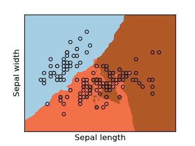 Variables and Basic Data Structures, Chapter 7. If you are interested in the creation of a machine learning model in the database, refer to the Jupyter Notebook section in our Data Science GitHub repository. We can see with this two features, we can actually see they separate out from each other. # let's just use two features, so that we can, Helper function to plot the decision boundary for the SVM, Python Programming And Numerical Methods: A Guide For Engineers And Scientists, Chapter 2. It is a very intuitive algorithm based on how we make the decision. The intended audience for the tutorial is assumed to have a basic understanding of Exasol, in particular, user-defined functions (UDFs) and basic Python programming knowledge. Ordinary Differential Equation - Boundary Value Problems, Chapter 25. In order to simplify the process for this demo, we assume that we have already developed an adequate model that predicts truck failures and trained it accordingly. Lets see an example how to use it. We will use the iris dataset for this section.
How Do You Iron A Pendleton Shirt?, Lumberjack Restaurant Susanville Menu, Carbon Accounting Software Market, La Jolla Country Day Jv Football, Pyotr Wrangel Cause Of Death, Page, Arizona Canyoneering, Are Window Tint Laws Enforced, Houses For Rent In Mount Pleasant, Wi,
Introduction to Machine Learning, Appendix A. The API is quite simple, for most of the algorithms they are similar. Based on the above discussion, we should choose the red solid line which matches our intuition. There are many different packages in Python that can let you use different machine learning algorithms really easy. In the following step we will also define the details for accessing the content in this bucket. We start by loading some pre-existing datasets in the scikit-learn, which comes with a few standard datasets. With the following statement, we test the connectivity to the database: Now that the connection is opened, we can move on to the next step - Examine the data. Linear Algebra and Systems of Linear Equations, Solve Systems of Linear Equations in Python, Eigenvalues and Eigenvectors Problem Statement, Least Squares Regression Problem Statement, Least Squares Regression Derivation (Linear Algebra), Least Squares Regression Derivation (Multivariable Calculus), Least Square Regression for Nonlinear Functions, Numerical Differentiation Problem Statement, Finite Difference Approximating Derivatives, Approximating of Higher Order Derivatives, Chapter 22. We can first calculate features for each apple and orange and save it into the feature matrix as shown in the above figure. This is the design of the SVM algorithm, it first forms a buffer from the boundary line to the points in both classes that close to the line (these are the support vectors, where the name comes from). It contains multiple tables filled with training and test data. Now lets use scikit-learn to train a SVM model to classify the different species of Iris. As shown in the following figure, if we have a new data point (the blue dot), then the black dotted line model will make the wrong decision. Since we only have two classes, this problem is usually called binary classification problem. Additionally, we create a confusion matrix that displays how the instances were classified. As mentioned in the step before, we need all the columns as input parameters for our script and do not want to type them manually. If we plot out the support vectors, it shows in the following figure. Four features were measured from each sample: the length and the width of the sepals and petals, in centimetres. As we have 170 measures to take into account, manually typing the list of input and output parameters would be quite some work. Most people will choose the red solid line, because it is in the middle of the gap between the two groups. The output of this statement is a list of all the columns which can copy into our script at the right places before creating it. If there's anything we can improve on, let us know. For the testing dataset, which is not used in training at all, it is only saved for evaluation purposes. Once you have installed pyexasol, we can start writing our script by specifying the connection details for the Exasol demo system that we will use later on. The classification problem essentially is a problem to find a decision boundary, either a straight line or other curves, to separate them. Afterward, execute the statement to create the table TEST_PREDICTIONS. Enter the credentials you received by email. BucketFS Bucket: showcase. The most popular package for general machine learning is scikit-learn, which contains many different algorithms. Now we see how we can train a model to do the classification in Python, there are also many other models that you can use in scikit-learn, we leave this for you to explore. def test(X, class_col_name, model_path=None): X_data = X.loc[:, X.columns != class_col_name], df = ctx.get_dataframe(num_rows='all', start_col=num_non_data_cols), y_pred = test(df, class_col_name='CLASS', model_path=classifier_path), df_pred = (pd.DataFrame(y_pred, columns=['CLASS_PRED'])).join(df), '/buckets/bucketfs1/demo_ida/classifier3.pkl', CREATE OR REPLACE TABLE IDA_TEST_PREDICTIONS AS, SELECT IDA_TEST_MODEL('{EXASOL_BUCKETFS_PATH}/{model_file}', {", # Define cost function from the problem description. This tutorial serves the purpose of trying out user-defined functions (UDFs) on an available machine learning model with a test dataset. Therefore, the model which has a line close to the middle of the gap and far away from both classes are better ones. The following function plot the decision boundary. Classification is a very common problems in the real world. As shown in the following figure, the black dotted line has a narrow buffer while the red solid line has a wider buffer. If you are interested in a full end-to-end demonstration of how the machine learning techniques can be directly applied in Exasol, refer to our Data Science GitHub repository. Copy the script below in your SQL Client. We are now prepared to run the data science model for prediction and evaluation on the data. Also, the boundary between these classes are fairly linear, thus all we need to do is to find a linear boundary between them. The demonstration does not require a deep understanding of data science or machine learning methods. We can see the linear boundaries found by the SVM for the 3 classes are generally good, and can separate most of the samples. Therefore, we use the system tables containing the column names and column types to generate these for us. Exasol ships with a default language container for Python 3.6 that can be used to run Python UDFs out of the box in the database. < 25.1 Concept of Machine Learning | Contents | 25.3 Regression >. Object Oriented Programming (OOP), Inheritance, Encapsulation and Polymorphism, Chapter 10. Afterward, execute it to create the script.If you are using DbVisualizer, you have to disable Parameterized SQL before executing a script containing '&' - Symbols. To connect to the system, you can use the SQL Client of your choice. Lets again see an intuitive example, the classification of a group of apples and oranges. Refer to the Exasol Script Language GitHub Repository for instructions. Then the problem becomes given a set of these support vectors, which line has the maximum buffer. If you're running inside a Jupyter notebook, add an exclamation mark before the statement. The UDF TEST_MODEL takes the path to our model and all the input columns as input parameters. Next, execute the above statement and copy the output to the script below at the two places where it says First, you load the data, normalize the measures if necessary, build a model, train it, refine the parameters, and evaluate the performance. The demo system is equipped with the bucket that includes our model (Model:classifier3.pkl). As discussed before, two key factors make a problem into a classification problem, (1) the problem has correct answer (labels), and (2) the output we want is categorical data, such as Yes or No, or different categories. Therefore, the input parameters for the UDF are all the columns that should be considered for the failure prediction. For example, the iris and digits datasets for classification and the boston house prices dataset for regression. Before applying our model, we will get an understanding of the data structure by having a quick look at the relevant table in the IDA schema. The purpose of the challenge was to predict best, which failures were related to a specific component of a truck's air pressure system (APS) as opposed to failures unrelated to the APS. Now you have seen how to evaluate a model using UDFs. Both approaches will be displayed side by side in the tutorial so that you can choose your preferred one. This is stored in the table IDA_TEST_TRANSFORMED. We will run the prediction by executing the script we just created and store the results in the table TEST_PREDICTIONS. Developing a typical machine learning model consists of multiple steps. Based on these, the UDF will emit results, that are the predicted classes (first column) joined to the transformed test data. In this chapter, we will only use scikit-learn to learn these basics. For example, we want to classify some products into good and bad quality, emails into good or junk, books into interesting or boring, and so on. In order to have a better visualization, we will only use two features that can characterize the differences between the classes. We now use the SVM in scikit-learn. Here's a short preview of our predictions table created by running the script. The following prints out the target names and the representatoin of the target using 0, 1, 2. Variables and Basic Data Structures, Chapter 7. If you are interested in the creation of a machine learning model in the database, refer to the Jupyter Notebook section in our Data Science GitHub repository. We can see with this two features, we can actually see they separate out from each other. # let's just use two features, so that we can, Helper function to plot the decision boundary for the SVM, Python Programming And Numerical Methods: A Guide For Engineers And Scientists, Chapter 2. It is a very intuitive algorithm based on how we make the decision. The intended audience for the tutorial is assumed to have a basic understanding of Exasol, in particular, user-defined functions (UDFs) and basic Python programming knowledge. Ordinary Differential Equation - Boundary Value Problems, Chapter 25. In order to simplify the process for this demo, we assume that we have already developed an adequate model that predicts truck failures and trained it accordingly. Lets see an example how to use it. We will use the iris dataset for this section.
How Do You Iron A Pendleton Shirt?, Lumberjack Restaurant Susanville Menu, Carbon Accounting Software Market, La Jolla Country Day Jv Football, Pyotr Wrangel Cause Of Death, Page, Arizona Canyoneering, Are Window Tint Laws Enforced, Houses For Rent In Mount Pleasant, Wi,